RFM Viewing Geometries

RFM Viewing Geometries |
| |
25MAR24 | ||
The homogeneous case, suitable for representing lab measurements or horizontal paths in the free atmosphere, is trivial and, apart from temperature, pressure and composition, the only additional parameter required to define the 'view' is the path length. For such cases, usually the only calculation required is of path transmittance.
The plane-parallel representation treats the atmosphere as a set of horizontal layers. The viewing direction is specified by secθ (equivalent to an 'air mass factor'), where θ is the angle with respect to the vertical. Provided that θ represents the viewing angle at the surface rather than the satellite, this generally provides an acceptable simulation for nadir-viewing instruments, at least for secθ≲2 (or θ≲60°)
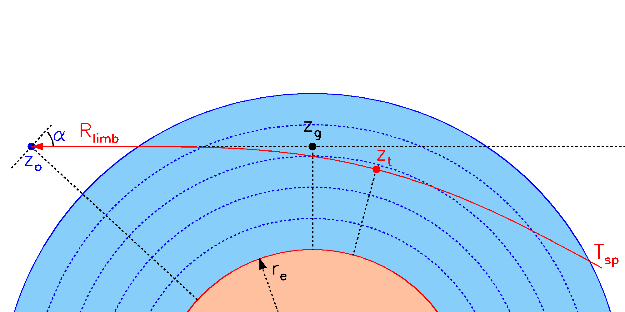
The circular atmosphere is the most general case, allowing for the curvature of the earth, refraction and field-of-view convolution. The curvature is assumed fixed over the path length, i.e., profile levels forming concentric circles in the viewing plane. Viewing directions can be specified either as tangent heights (for limb-viewing) or elevation angles α relative to the observer horizontal (suitable for geometries which intersect the surface or upward views from within the atmosphere), in which case the observation altitude is also required.
In principle, nadir-views for the circular (α=-90°) and plane-parallel (θ=0°) atmospheres are identical, refraction and curvature having no effect; however small differences arise from the different path integration methods.
When running the RFM, the basic viewing geometry is specified in the
driver table by the appropriate flag
in the *FLG section and further
details in the sixth primary section
(labelled
*TAN,
*GEO,
*ELE,
*SEC or
*LEN)
Homogeneous Path
|
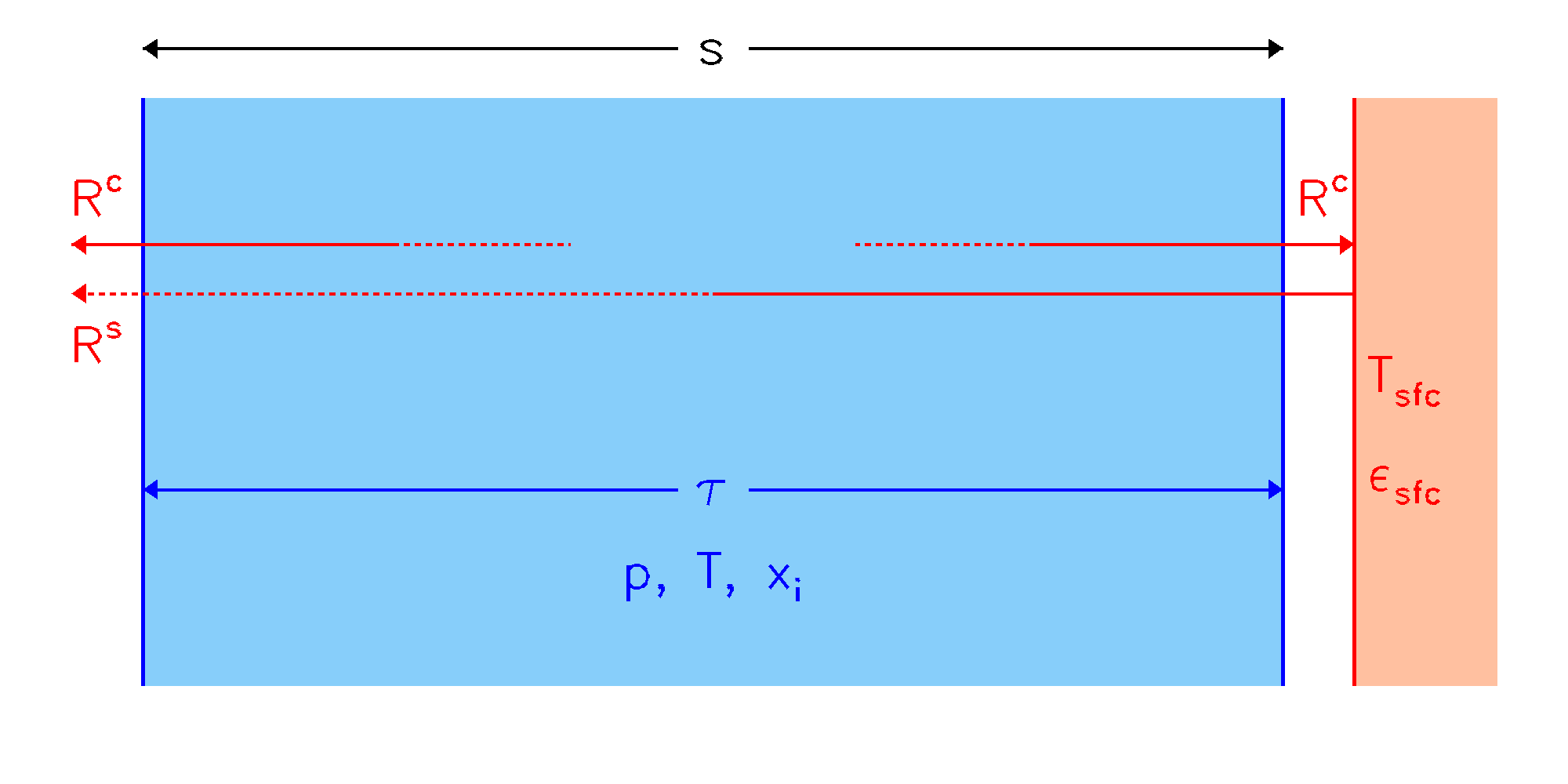
| The user specifies temperature T, pressure p, volume mixing ratios xi of absorbing molecules and a path length s, from which τ, representing transmittance, absorption or optical depth is calculated. A radiance R can also be calculated (left of plot) which will be the sum of the cell emission Rc and the attenuated emission Rs of a background surface of temperature Tsfc. For surface emissivity εsfc < 1, Rs will also include a reflected component of Rc. |
It is assumed that most homogeneous path calculations will be for transmittance
but radiance can also be calculated. Then it is necessary to consider the
boundary condition at the remote end of the path. By default, the RFM assumes
a space view, but by using the
SFC flag and
*SFC section, any boundary
temperature and emissivity can be specified.
Plane Parallel
|
|
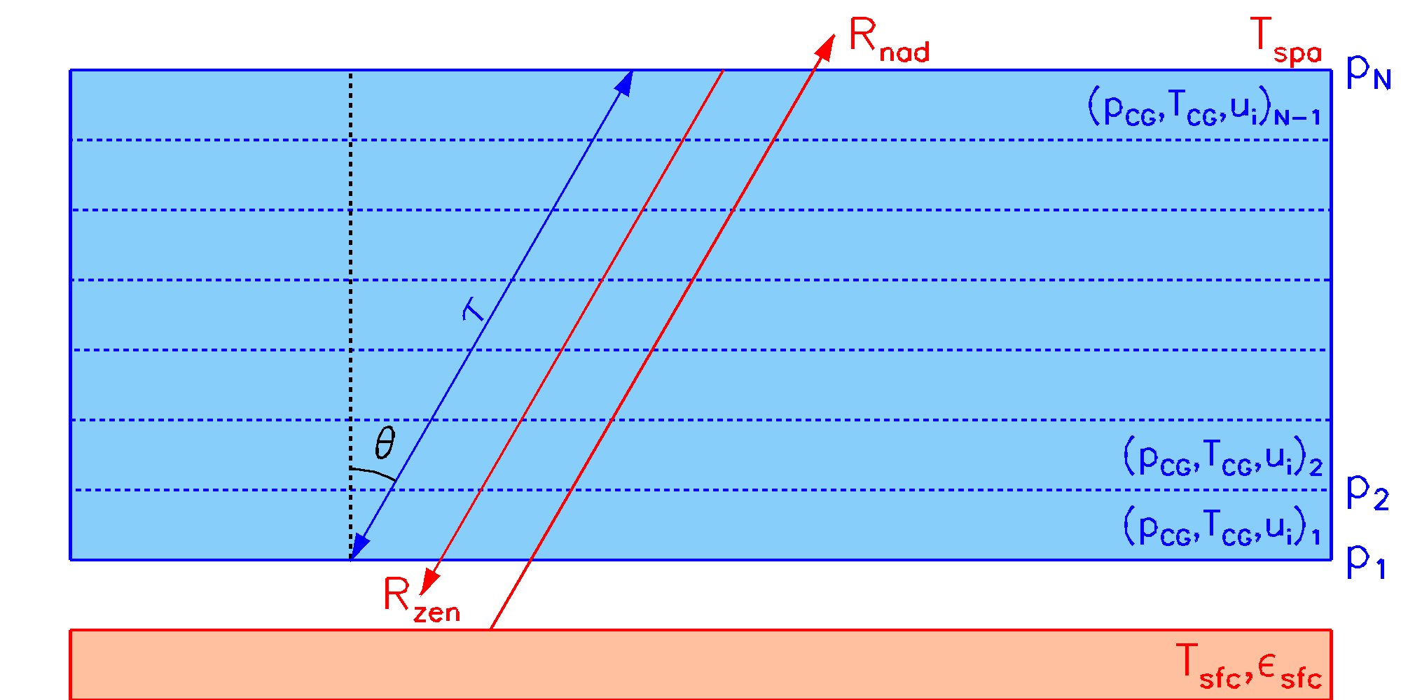
The user selects either a Zenith or a Nadir view and specifies an air-mass factor secθ, where θ is the angle of the path to the vertical (secθ=1 for a vertical path). The user specifies atmospheric profiles of temperature Tj and volume mixing ratios xi,j of absorbing molecules at N pressure levels pj. From this the RFM defines N-1 layers, each characterised by Curtis-Godson equivalent parameters TCG, pCG and partial columns ui. The upward-looking radiance (at the surface) Rzen is initialised with the space background radiance Tspa (usually negligible except for microwave region). The downward-looking radiance (from space) Rnad, for a non-reflective surface is initialised with the surface emission. Both calculations then proceed though the atmosphere treating each layer as a homogeneous path. (For a reflective surface there is first a downward radiance calculation, of which a reflected component is added to the surface emission.) Atmospheric transmittance, absorption or optical depth, represented by τ, is the same for both nadir and zenith directions. |
An advantage of this assumption is that Curtis-Godson equivalent paths can be calculated analytically from the atmospheric profile values, and (for any given absorber) CG mean pressure and temperature are independent of viewing angle.
In principle effects such as refraction and field-of-view convolution could be applied to such an atmosphere, but the RFM only applies these for the circular geometry.
For basic ray calculations through a plane-parallel atmosphere it is necessary to specify the following in the driver table
If an observer altitude is specified within the atmosphere
(OBS flag) then the viewing geometry
may alternatively be specified by an elevation angle α, in degrees,
relative to the horizontal. This is done by replacing the
section label
Flux calculations (FLX Flag), which
involve integration over solid angle, also use the plane-parallel assumption.
Circular Geometry
|
|
The ray-path, shown in red can be specified in three ways:
The atmosphere is defined in the same way as the plane parallel atmosphere, although in this case the Curtis-Godson equivalent parameters are derived for each path separately. |
The ray path is specified according to how the *TAN section of the driver file is labelled.