The Scattering Reference Forward Model (SRFM) is a general-purpose one-dimensional line-by-line radiative transfer code. Its main purpose is to provide a versatile Python package to solve the radiative transfer problem with particle scattering calculations from Mie theory. Compared to existing radiative transfer codes, the SRFM provides a user friendly and modular environment with flexibility for the user to setup their own atmospheric conditions. For example, the code can be used to calculate radiative transfer for clear sky atmospheres (a purely gaseous atmosphere) and include particle scattering properties layers without. The SRFM implements two existing radiative transfer codes - the Reference Forward Model (RFM) and Discrete Ordinate Radiative Transfer (DISORT). One particular application of the code is the analysis and simulation of top-of-atmosphere volcanic cloud spectra.
The code can be installed from PyPI by:
pip install srfm
The source code is maintained on Github:
https://github.com/eodg-oxford/srfm
The documentation to the code can be accessed here:
https://srfm.readthedocs.io/en/latest/
The code is maintained primarily by Antonin Knizek (antonin.knizek@physics.ox.ac.uk). Alternatively contact Roy Grainger (roy.grainger@physics.ox.ac.uk).
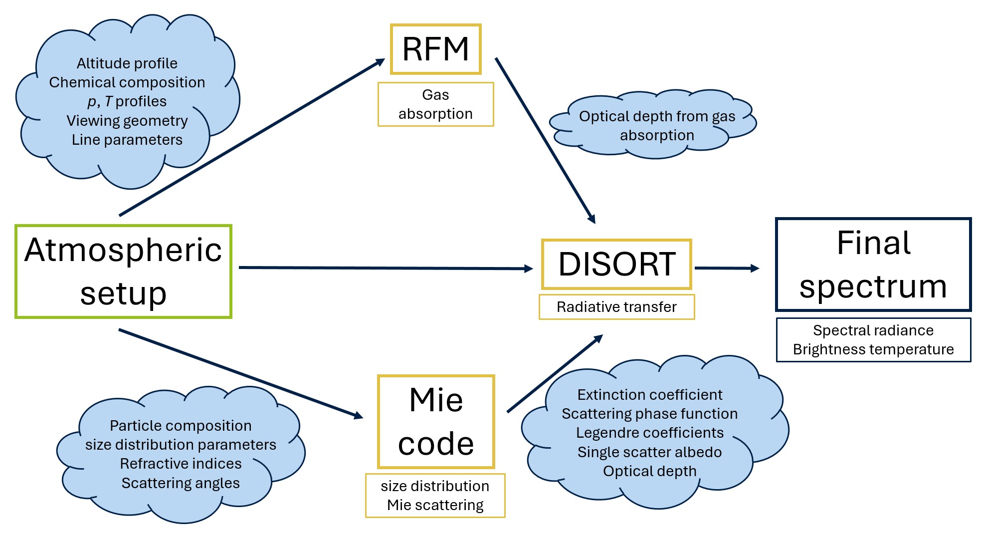
The SRFM is a Python package. The code implements the Reference Forward Model and the Discrete Ordinate Radiative Transfer. The package has the following structure:
The code, when used as a radiative transfer model, starts with an atmospheric setup by the user through a driver table. Parameters are then passed to the RFM part of the code, which calculates gas absorption, emission and the resulting optical depths. Simultaneously, the code calculates the optical properties resulting from the presence of scattering particles, such as optical depth, extinction, single scattering albedo and the phase function. All these properties are then passed onto DISORT, which calculates the multiple scattering radiative transfer throughout the atmosphere. A result from the code is a radiance spectrum or brightness temperature if requested.
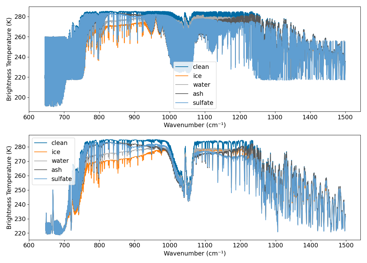
This example plot shows two panels. Each panel contains five brightness temperature spectra calculated with the SRFM. The spectra represent five different atmospheric scenarios. The top panel shows a result from a high resolution (0.001 cm-1) calculation. The bottom panels shows identical the same spectra, but convolved with the Infrared Atmospheric Sounder Interferometer instrument response function to show an example of what a real satellite instrument would see. In the figure, the label clean signifies a clear sky atmosphere with a standard mid-latitude profile. The same atmosphere was then taken and four different layers were inserted, respectively - an ash layer, a sulfuric acid layer, a water cloud and an ice cloud. The parameters of these layers were chosen arbitrarily to maximise the spectral difference and illustrate the influence of the presence of scatterers in the atmosphere. As is seen from the figure, the presence of each scatterer influences the spectrum in a specific manner. For instance, the presence of water and ice particles both create a slope in the spectrum between approximately 750 and 950 cm-1, albeit different in each case. On the other hand, the presence of sulfuric acid aerosol creates an opposite slope with three distinct features across both atmospheric windows (750–950 and 1100–1250 cm-1) in this plot. Ash creates a yet different distortion to the spectrum with a characteristic V-shape over the two atmospheric windows. This plot illustrates that high-resolution calculations can be used to distinguish the type of scatterer as well as their respective mass loading, effective radius, size distribution or type (e.g. different volcanic ash types will have different refractive indices and therefore a characteristic effect on the spectrum.)
Maintained by Don Grainger